Consumer Equilibrium and Utility Analysis

The following are the topics discussed under Consumer equilibrium and utility analysis.

• Consumer behavior theory
• Utility analysis
• Marginal Utility Theory (Cardinal approach)
• Consumer Equilibrium
• Indifference curves analysis (Ordinal approach)

Consumer Behavior Theory

Under Consumer equilibrium and utility analysis, firstly, we discuss consumer bahavior theory. The consumer behavior theory describes,

how rational consumers make their purchasing decisions under the conditions and how they adjust their decisions when the given conditions change.

In other words, how consumers attain the equilibrium by purchasing a bundle of goods which gives them the maximum satisfaction/utility under the given conditions.

Firstly we will examine the theory of consumer behavior and the relationship between this theory and the theory of demand. The traditional theory of demand starts with a review of the demand of individual consumers because the market demand is assumed to be the summation of the demands of individual consumers.

Therefore, we will examine the behavior of an individual consumer. The behavior of the consumer is base on a few basic assumptions.

Assumptions of the Behavior of an Individual Consumer

It assumes that,

1. The consumer is rational
The rational consumer always plans to spend his income to attain the highest possible satisfaction (utility) given his income and market prices of commodities. So this is known as the ‘axiom of utility maximization.’

2. The consumer has full knowledge of all information relevant to his decision
For example, all available commodities, prices, income, etc.

Fundamental Approaches that Describe Consumer Behavior

The consumer goal is to maximize utility. So he must be able to compare the utility of various baskets of goods that he can buy with his income. There are mainly two approaches to analyze how this comparison can be made. They are:

1. Cardinal utility approach
2. Ordinal utility approach

Consumer equilibrium and utility analysis: Cardinal utility approach

According to the cardinal utility approach (cardinalist school), the utility derived by consuming commodities can measure. Moreover, Leon Walrus and some economists have suggested using a subjective measure known as ‘util.’

And also, Alfred Marshal and some others suggested using monetary units. For example, the amount of money a consumer is willing to pay for another unit of the commodity.

The cardinal utility approach describes the Marginal utility theory.

Consumer equilibrium and utility analysis: Ordinal utility approach

According to the ordinal utility approach, consumers cannot measure the utility using any objective unit of measurement because the utility is a subjective phenomenon. According to them, although utility cannot be measured, consumers can rank the various goods/baskets of goods based on the level of satisfaction derived by each of those goods or baskets of goods.

After ranking various bundles of goods, a consumer can buy the bundle that gives him the highest satisfaction.

Two main theories describe consumer behavior based on the ordinal utility approach.

1. Indifference curves analysis
2. Revealed preference hypothesis

Finally, we can confirm according to the cardinal utility approach utility can be measured, and in the ordinal utility approach, the utility can’t be measured. But it can be ranked to various levels.

Concept of Utility and Utility analysis

Consumer equilibrium and utility analysis are interconnected concepts. So let’s consider utility analysis.

Utility can define as, Refers to the power or the property of a commodity to satisfy human needs.

For example: to alleviate hunger can have foods, to quench thirst can have a soft drink, tea or coffee, etc

Utility,

• is the want satisfying power.
• derived by the consumer from a commodity depends on the intensity of desire.
• of many commodities depends on the availability of complementary goods
• is ethically neutral, is free from moral values and social desirability.

Utility function describes the relationship between utility and the factors that determine the utility.

The physiological and psychological make-up from person to person is different. Therefore the utility derived by consuming a commodity varies from person to person.

Hence there may be several factors affecting the satisfaction of the individual consumer. Some of them cannot be identified and measured.

Therefore, to define the utility function, economists take into account only the measurable factors. They assume that other factors remain constant. Accordingly, in the utility analysis, economists take into account only a few factors, including quantities of commodities, income, and prices of commodities.

Consumer Equilibrium and Utility Analysis: Utility Function

In utility analysis, it is important to derive the utility function. When income and prices of commodities remain constant, the utility or level of satisfaction depends on the quantities of goods consumed.

U_i = f(q_i),               i = 1. . . . n             (1)

U_i  = the level of utility

q_i  = the quantity of i th commodity

f   = the shape of functional relationship

n   = number of commodities

When all n commodities consume simultaneously, total utility will be sum of the utilities derived by individual commodities.

U = U₁+ U₂………..+ Un                                         (2)

Substituting equation (1) in to (2)

U = f₁(q₁)+ f₂(q₂)+…….+ f_n(q_n)

This can be simplified as

U = F (q₁,q₂…..q_n)                                                  (3)

This is called ‘utility function.’

A utility function defines the relationship between total utility and quantities of different goods consumed at a time.

However, the utility function can present in different ways, like an algebraic equation, as a mathematical model, as a schedule, like a graph.

Utility function satisfy two conditions

Every consumer will have a utility function that shows his preference. So it is assumed that this function satisfies two conditions.

1. It is a single-valued function

This means that the consumer will get only one level of satisfaction, not two or more when he consumes a given quantity of different goods. The level of satisfaction changes if and only if the amount of at least one commodity is changed.

2. It is a continuous function

This means that there exist first and second-order partial derivatives of the utility function for each good.

First-order partial derivatives can be derived from utility function (3) as follows:

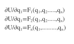
A partial derivative of the utility function can interpret as the change of total utility by consuming one more extra unit of a given commodity keeping the number of other commodities constant.

In economic the partial derivatives of a utility function are called marginal utilities of commodities.

Example: If ten units of a given commodity give 50 units of utility and if 11units give 55 units of utility, then the MU of the 11th unit of the commodity is 5.

Consumer Equilibrium and Utility Analysis: Marginal Utility Theory

This theory is based on the cardinal utility approach, and the analysis is based on certain assumptions.

1. Rationality

The consumer goal is to maximize utility by his given income. The consumer must spend his income to get the highest utility. So to the consumer must be rational.

2. Cardinal utility

According to some economists called Gossen, Jevons and Walrus utility derived by consuming commodities can measure. They suggest a subjective measure known as ‘util’ to measure utility.

However, Alfred Marshall suggested using monetary unis. According to him, a unit of a commodity is equal to the amount of money which consumer is willing to pay for that unit.

The utility is a subjective phenomenon. So different to agree with cardinal utility.

3. Constant marginal utility of money

Marginal utility (MU) of money remains unchanged. This assumption was required because monetary units used to measure utility by Marshall. Any standard unit of measurement must remain constant. If the measuring unit change, it will become an ‘elastic ruler.’

Sometimes this assumption away from the truth. In fact, this is one of the highly criticized assumptions together with cardinal utility assumption later.

4. Independent utilities

According to the Cardinalist school, consumption of a product is a function of the same product. So it does not depend at all upon the quantities consumed from other goods.

According to Marshall utility of the variety of goods together. Later this assumption excluded. So this is not realistic.

5. Diminishing marginal utility

In diminishing, marginal utility consumer increases the consumption of good and services.

As mentioned, MU is the change in total utility. as a result change of one unit of a given commodity keeping the quantities of other commodities constant.

6. Introspection method

The marginal utility of another person can judge with the help of self-observation.

The Law of Diminishing Marginal Utility

As the axiom of diminishing marginal utility describes when the number of units of a commodity consumed by an individual increases within the given time period, marginal utility (MU) decreases gradually.

Because of this behavior of MU, total utility (TU) increases with the increase of the quantity. TU, however, increases only up to a certain level of consumption.

If the consumption exceeds this level, TU will decline. This shown by the diminishing of the slope of the TU curve.

The slope of the TU curve represents the MU. Hence, diminishing the slope of TU reveals that the MU of successive units is diminishing.

Qx	0	1	2	3	4	5	6	7
TUx	0	10	18	24	28	30	30	28
MUx	-10	8	6	4	2	0	-2	

Graphically, this behavior of total and marginal utility can be shown as follows:

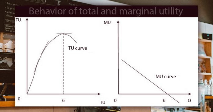
The behavior of the total and marginal utility

Up to the 5th unit, the total utility has increased. Beyond the 5th unit, it has started to decrease. Even within the increasing range of TU, it increases at a decreasing rate.

The slope of the tangent at any point on the TU curve gives the MU of that unit. The slopes of tangents have decreased. Thus, MU gradually decreases, and it has become zero in the 6th unit. In the decreasing range of TU, MU is negative.

At the consumption level that MU is zero, the consumer gets maximum TU. Extra unit beyond this point will not increase his utility.

Hence, a rational consumer will stop consuming commodities at the point where MU is zero. This is because a rational consumer consumes a commodity to the extent that it gives him maximum satisfaction.

Conditions for the law of diminishing marginal utility

The law of diminishing marginal utility is valid only when certain conditions are satisfied.

• Consumption is continuous: there is no time gap in the process of consumption.
• The taste or preference of the consumer remains unchanged during the period of consumption.
• All units of the commodity are homogeneous in size.

For example, suppose that the consumption function for a commodity of a consumer is given by,

Q = 100Q- Q² How many units of the commodity the consumer buy?

Consumer Equilibrium

In Consumer equilibrium and utility analysis, firstly, we considered utility analysis. Now we move to consumer equilibrium.

In the consumer equilibrium, we examine how a consumer allocates his given income among the various goods and services that he wants to consume.

However, the consumer cannot consume all that he wants to consume. That is because his disposable income is not sufficient. This means that the consumer has to maximize his utility subject to the income or budget constraint.

Hence, consumer equilibrium can consider as a problem of maximizing utility subject to the income constraint. Moreover, it is a problem of constrained utility maximization.

Example of consumer equilibrium

A consumer needs several goods and services for consumption. Firstly, we begin with the simple model of a single commodity. Let’s consider it as X. Suppose that his income is M and the market price of X is Px.

commodity – X
income – M
market price of X – Px

In this situation, he can either buy commodity X by spending all his income. Otherwise, he can entirely keep his money income with him.

We assume that utility can measure by use of monetary units. The utility of a unit is equal to the amount of money that the consumer is willing to pay for that unit.

the utility of a unit = amount of money that the consumer is willing to pay for that unit

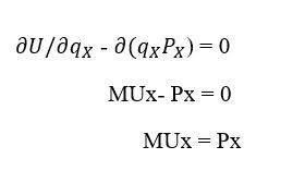
In these conditions, the consumer is in equilibrium when the marginal utility of X equal to the market price of X.

MUx = Px

If MUx > Px, the consumer can increase his satisfaction by purchasing more of X.

If MUx < Px, he can increase his satisfaction by cutting down the quantity of X and keeping more of his money with him.

This adjustment will continue up to the point where MUx = Px.

Derivation of the equilibrium conditions

We can derive this equilibrium condition mathematically as follows:

The utility function is U = f(qx)

If the consumer buys qx units of X, his expenditure would be qxPx. For the equilibrium, he seeks to maximize the difference between utility and his expenditure (the difference between U – qxPx).

The necessary condition for the maximization of this function is that the partial derivative of the function
with respect to qx be equal to zero.

We can generalize this condition for ‘n’ commodities as

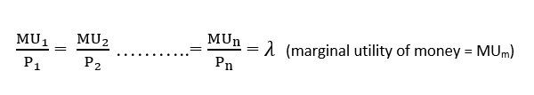
marginal utility of money

subject to the constraint of P₁Q₁ + P₂Q₂ + ……+ P_nQ_n = M

Consumer Equilibrium and Utility Analysis: Law of equi-marginal utility

The above conditions are the equilibrium conditions for the maximization of utility under the income/budget constraint. The above relationship shows the maximization of utility under income constraint.

In this situation, the consumer should allocate his income among various commodities. So in such a way that the last unit of money spent on each commodity brings him the same marginal utility.

This is known as the law of equi-marginal utility or the law of commodity substitution. For consumer equilibrium, this condition is very important.

If we take into account a two-commodity case, the equilibrium condition can be written as:

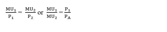
The ratio of marginal utilities of two commodities must be equal to the ratio of their prices.

In the two commodity case if MU₁/P₁ > MU_2/P₂. This means that consumer gets higher utility per unit of money spent on commodity 1 than commodity 2. In such situation consumer will buy more of commodity one spending more on it. As a result, MU₁ will decrease as such the ratio MU₁/P₁ decreases which will be eventually equal to the ratio of MU₂/P₂. In this way, the consumer attains the equilibrium.

If we summarize the above there are two conditions for equilibrium.
The necessary condition is MU1/P1=MU2/P2= MUm.
The sufficient condition is, P₁Q₁ + P₂Q₂ = M

Derivation of the law of demand and demand curve

Consumer demand and the demand curve can derive based on the axiom of diminishing marginal utility.

The law of demand says that there is a negative relationship between the quantity demanded and its price, under the assumption of ceteris paribus.

Based on this condition, we can build the demand schedule of a consumer. The demand curve shows the amount of a commodity that consumer plans to purchase at various prices.

As in Figure 1, when the quantity of the commodity X increases, the total utility also increases up to a certain point. Still, at a decreasing rate MUx declines continuously, and it becomes negative beyond the quantity that gives him the maximum utility (Fig. 2). If the utility measure in monetary units, at the equilibrium MUx, = Px.

Suppose quantity X1 gives the MU1 level of marginal utility. According to the utility theory at the consumer equilibrium MU1 = P1.
Thus, at price P1, the consumer will buy X1 quantity. Similarly, at X2, MU2 = P2 and consumer will buy X2 quantity at a price P2 and so on.

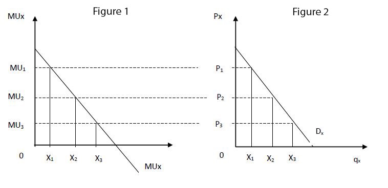
By converting the positive segment of the MU curve into another two-dimensional plane which shows the demand curve can derive.

Hence the consumer demand curve is identical to the positive segment of the MU curve. The negative part of the MU curve does not a part of the demand curve. It is because negative quantities do not make sense in economics.

Critique of the Cardinal Approach

Throughout this article discussed a wide range of consumer equilibrium and utility analysis. As the oldest theory of consumer behavior, cardinal utility approach made a valuable contribution to the theory of economics. The theory describes consumer equilibrium when the consumer income and prices of commodities given.

Further, it was successfully derived the demand curve and establish the law of demand. However, there are several limitations to the cardinalist approach.

1. This approach based mainly on the assumption that utility can measure.

Walrus suggested using a subjective measure known as util. Marshal used monetary units. However, the utility is a subjective phenomenon. It cannot measure objectively by use of any measure. This assumption gives serious doubt about the entire analysis.

2. The assumption of the constant utility of money is also unrealistic.

Marshal used this assumption because he measured utility using monetary units. The absolute value of any measuring unit must keep constant. However, this assumption does not hold in practice.

Because of the change of money or nominal income, as well as real income, affect the marginal utility of money. The change in utility of money affects the demand for commodities.

3. failed to isolate the total effect of a price change into the substitution and income

Another serious drawback of the approach is that it failed to isolate the total effect of a price change into the substitution and income effects. So the demand curve slopes downward because of these two effects.

But, since the assumption of constant marginal utility of money, this approach was unable to take into account the change of real income.

When the price of a commodity change, the real income of the consumer change. Change of real income causes to change the demand. This is the income effect of price change.

Since the assumption of constant marginal utility of money, this approach could not take into account the income effect of price change.

4. failed to analyze the availability and the demand for inferior goods and Giffen goods.

Because of this drawback, this approach failed to analyze the availability and the demand for inferior goods and Giffen goods.

The goods which have larger negative income effect relative to the positive substitution effect of price decrease identify as the Giffen goods.

The goods which have a smaller negative income effect relative to the positive substitution effect of price decrease identify as the inferior goods.

Since this theory was not capable of isolating substitution and income effect of price change, it could not identify the Giffen and inferior goods.

5. The axiom of diminishing marginal utility is a psychological law.

So it cannot be applied for all.

Then we done marginal utility theory based on the cardinal utility approach. This theory is based on certain assumptions, and we identified what those are. Then we did the law of diminishing marginal utility. Diminishing marginal utility describes when the number of units of a commodity consumed by an individual increase within the given time, and marginal utility (MU) decreases gradually. Then we learned assumptions of diminishing marginal utility.

After discussing the law of diminishing marginal theory, we understood consumer equilibrium. In the consumer equilibrium, we examined how a consumer allocates his given income among the various goods and services that he wants to consume. Then we did an example of consumer equilibrium. Secondly, we derive equilibrium conditions. There are two conditions for equilibrium. Then we derived the law of demand and demand curve. Finally, we examined the critiques of the cardinal approach.

Questions

Conclusion

So let’s just summarise what we have done till now. Firstly we discussed what consumer behavior theory is. In the consumer behavior theory, we identified how consumers attain the equilibrium by purchasing a bundle of goods, which gives them the maximum satisfaction/utility under the given conditions.

To understand consumer behavior theory most clearly, we need to understand what is the utility. Before learning about utility theory, we identified two theories that describe consumer behavior. They are the Cardinal utility approach and the Ordinal utility approach. In the cardinal utility approach, we must know about diminishing marginal utility analysis and equi-marginal utility. And also, in ordinal utility approach must learn about indifference curve analysis. From this article, we consider about cardinal utility approach.

Then we learned the Concept of Utility and Utility analysis. Under this heading, we discussed definitions for utility, what is utility function, how can we derive utility function and two conditions of the utility function.

Did I miss anything? Let me know by leaving a comment.