
Theory of Cost: Money value of inputs is called the cost of production. Let’s discuss.
Laws of production are expressed in terms of physical quantities Example: labor, capital, and output in terms of units.
However, business decisions regarding production are taken on the basis of the money value of inputs and the money value of output.
So money value of inputs is called the cost of production and the money value of output is referred to as sales revenue.
Theory of Cost: Cost Concepts
A variety of cost concepts are used in economic analysis and firm’s decision making. In general cost, concepts are classified into three categories.
- Accounting cost concepts
- Analytical cost concepts
- Policy related cost concepts
Accounting Cost Concepts
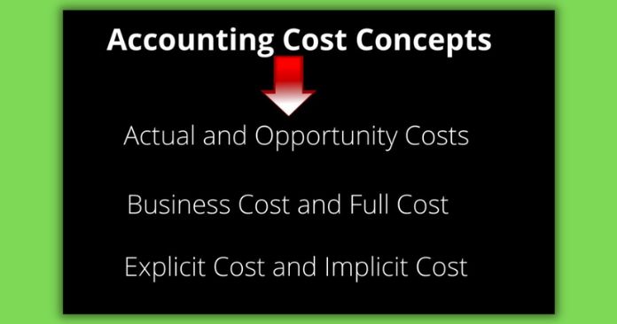
- Actual and Opportunity Costs
Actual cost is the expenditures that are actually incurred by the firm in payment for the use of resources obtained from the outside such as payments for labor, material, plant, traveling and transport, fuel, and so on.
Opportunity cost is the losses of income due to opportunity forgone. Opportunity cost is also called economic cost. Opportunity cost comes under economic rent. Economic rent is the difference between the actual earnings and the opportunity cost (expected returns from the second-best alternative use of the resources).
- Business Cost and Full Cost
Business cost includes all the expenses which are incurred carrying out the business. Business cost includes all the payments and contractual obligations made by the firm and depreciation.
The concept of full costs includes opportunity cost and normal profit. Normal profit is a necessary minimum earning in addition to alternative cost, which a firm must get to remain in its present occupation.
- Explicit Cost and Implicit Cost
Explicit cost is those which are actually incurred by the business firms and are entered in the books of accounts.
The costs which do not take the form of cash outlays are known as implicit costs. Implicit cost is similar to opportunity cost. The implicit cost includes implicit wages, implicit rents, implicit interest, and so on.
Analytical Cost Concepts
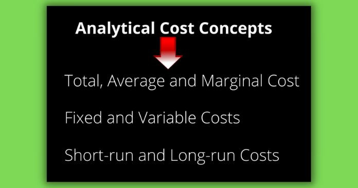
- Total, Average and Marginal Cost
Total cost (TC) shows the total resources used in the production of goods and services. It includes total outlays of money expenditure both explicit and implicit on the resources used to produce a given output.
Average cost is the ratio between total cost (TC) and total output (Q).
Total cost – (TC)
Total output – (Q)
AC = 𝑇𝐶/𝑄
Marginal cost (MC) is the addition to the total cost of producing one additional unit of product.
MC = ∆𝑇𝐶/∆𝑄
- Fixed and Variable Costs
The costs that do not vary over a certain level of output are known as fixed cost. Variable costs are those which vary with the variation in the total output.
- Short-run and Long-run Costs
A short-run cost includes fixed cost and variable cost. In the long run there is no fixed cost. All the costs are variable cost.
Policy Related Cost
Private and Social Costs
- Private costs are those which are actually incurred by the firm on the purchases of goods and services from the market. For a firm, all the actual costs include both explicit and implicit are private cost.
- Social cost implies the cost which a society bares on account of the production of a commodity. Social cost includes both private cost and external cost (positive and negative externalities).
Theory of Short-run Cost
Short-run total cost (TC) consists of fixed cost and variable cost.
TC = TFC + TVC
Where
TC = Total Cost
TFC = Total Fixed Cost
TVC = Total Variable Cost
Average cost = TC/Q = TFC/Q + TVC/Q
Marginal cost = ∂TC/∂Q
∂TC = ∂TFC + ∂TVC
∂TFC = 0
∂TC/∂Q = ∂TVC
MC = ∂ TVC
The Short Run Cost-Output Relationship
In the short-run production takes place under the laws of returns to variable input or the law of diminishing returns.
As long as output increases at an increasing rate, the cost of production increases at a decreasing rate, and when output increases at decreasing rate cost of production increases at a decreasing rate.
Graph (A)
Graph (B)
Graph (C)
Graph (D)
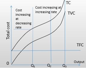
Cost-output Relationship in Short- run
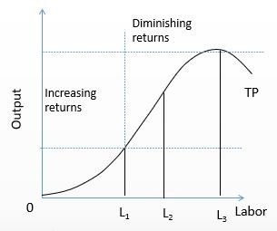
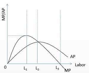
- The short-run cost output relationship is shown in graphs (a) and (b).
- As the graph (a) shows when labor increases from 0 to L1, output increases at an increasing rate.
- When labor is increased beyond OL1 output increases but at a decreasing rate and output is maximized at OL3.
- graph (b) shows, over the 0L1 range, TC increases at decreasing rate. The increase in TC at decreasing rate is indicated by the decreasing slope (∆𝑇𝐶/∆𝐿) of the TC curve. Similarly, the increasing TC at an increasing rate corresponds to the range of TP increasing at a diminishing rate.
- The trend of the relationship between cost and output proves the point that laws of returns to variable input in the form of the theory of cost.
Therefore, the short run theory of cost can be summarized as below.
(1) Total Cost (TC) increases with increase in total production (TP).
(2) As long as TP increases at increasing rate, TC increases at decreasing rate.
(3) When TP increases at a constant rate, total cost also increase at constant rate.
(4) When TP increases at decreasing rate, TC increasing at increasing rate.
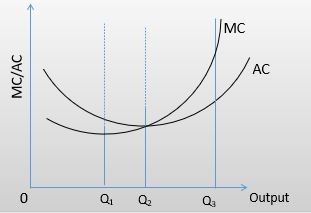
The Average and Marginal Cost Behavior
MPL goes on increasing until OL1 labor and MC goes on decreasing till the corresponding output Q1. MPL reaches its maximum at OL1 and MC reaches its minimum at the same level of output (0Q). As MPL begins to decline MC begins to rise.
Further, it can be observed from panels that as AP goes on increasing, AC goes on decreasing, where AP reaches its maximum, AC decreases to its minimum and when AP begins to decline, AC begins to rise.
Short-run Cost Functions and Cost Curves
The cost function of a firm is derived on the basis of the actual cost and production data of the firm.
Given the cost and production, the data cost function may take a variety of forms. It may be a linear, quadratic, or cubic cost function. The simple total cost functions which produce U-shaped average and marginal cost curves are at cubic polynomial form as given below.
TC = A + bQ – cQ2 + dQ3
A = Total Fixed Cost (TFC)
b,c and d = Parametric constants
The AFC, AVC, AC and MC can be derived from the total cost function.
AFC = 𝐴/𝑄
AVC = 𝑇𝑉𝐶/𝑄 = (𝑇𝐶−𝐴)/𝑄 = (𝑏𝑄−〖𝐶𝑄〗^2+ 𝑑𝑄^3)/𝑄
= b – cQ + dQ2
AC = 𝑇𝐶/𝑄 = (𝐴+𝑏𝑄− 𝑐𝑄^(2 )+ 𝑑𝑄^3)/𝑄
= 𝐴/𝑄 + b – cQ + dQ2
MC = 𝜕𝑇𝐶/𝜕𝑄 = b – 2cQ + 3dQ2
Long Run Cost-Output Relationship
In the long run, firms can hire more of both labor and capital, more of raw materials and other inputs, while technology remains constant.
The long run means the sum of short runs.
Long-run cost curves would be composed of a series of short-run cost curves.
Total Long-run Cost Curve (LTC)
At the beginning, the short-run total cost is given by STC1. Let the firm add another plant to its size in the short-run 2.
As a result, the firm’s TC increases, and increase in the cost increase the output.
When the cost of the second plant is added to the first one, the TC curve shifts upward from STC1 to STC2.
Similarly, we will get STC3 and STC4. LTC can get by drawing a curve tangent to the bottom of the STCs.
Long-run Total and Average Cost
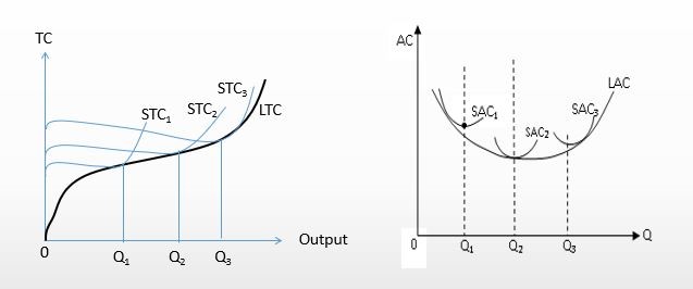
Theory of Cost: Long Run Average Cost Curve (LAC)
Note that the SAC of the second plant is lower than that of the first plant due to the economies of scale. However, when the third plant is added economies of scale is disappeared. Therefore SAC begins to rise.
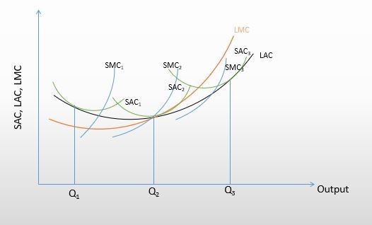
Long run average cost curve is drawn by drawing a curve tangent to SAC1, SAC2, and SAC3. The LAC is called as ‘envelope curve’ or planning curve as it serves as a guide to the entrepreneurs in their planning to expand the production in the future.
Theory of Cost: Long Run Marginal Cost Curve (LMC)
The long LMC is derived from the short run marginal cost curves. The procedure of derivation of LMC is exactly the same as the process of derivation of the LAC.
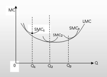
Theory of Cost: Optimum Size of The Firm in The Long Run
Long run cost curves LAC and LMC can be used to determine the optimum size of the firm.
The optimum scale of production is one that gives the most efficient utilization of resources –determined by the minimum LAC.
The optimum size is at the minimum cost, where LAC=LMC=SAC=SMC.
Rate the article if you learned something new from it.
⭐⭐⭐⭐⭐