
When a country’s currency loses value, most people expect trade to improve almost immediately. Exports become cheaper for foreign buyers, imports become more expensive at home — so the trade balance should swing positive right away, right?
Not quite. In practice, the opposite often happens first.
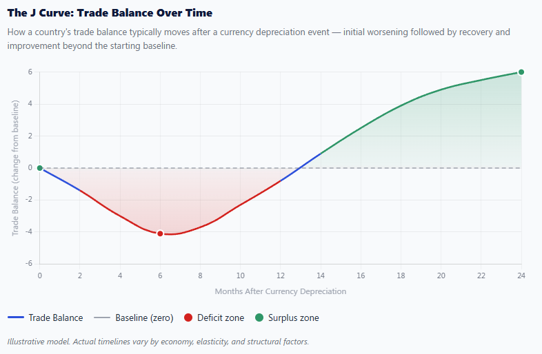
The J Curve is an economic concept that describes a counterintuitive pattern: after a currency depreciation, a country’s trade balance typically worsens before it gets better. When you plot this movement on a graph over time, the curve dips downward and then rises — tracing the unmistakable shape of the letter “J.”
Understanding the J Curve is essential for economists, policymakers, investors, and anyone trying to make sense of how exchange rates, international trade, and economic recovery interact. It explains why short-term pain often precedes long-term gain — and why governments must sometimes hold their nerve when the data looks discouraging.
Understanding the J Curve Effect
The J Curve effect refers specifically to the trajectory of a nation’s trade balance following a depreciation (or devaluation) of its currency. Rather than an immediate improvement, the trade balance follows a predictable three-part sequence:
- Initial deterioration — The trade deficit widens in the short run.
- Stabilization — The trade balance levels off as contracts expire and prices adjust.
- Improvement — Export volumes rise and import volumes fall, improving the trade balance over the medium to long term.
The reason this matters is that the J Curve challenges the instinctive assumption that cheaper exports automatically translate into better trade figures overnight. In reality, trade responds to price signals slowly — due to contracts, habits, and the time it takes for businesses and consumers to adapt.
Figure 1 · Classic Pattern
Why Does the J Curve Occur?
The J Curve occurs because of a fundamental mismatch between price effects and volume effects in international trade.
When a currency depreciates:
- Import prices rise immediately — Foreign goods cost more in domestic currency right away.
- Export prices fall for foreign buyers immediately — But overseas buyers need time to recognize this and change their purchasing behavior.
- Trade volumes adjust slowly — Existing contracts, supply chains, and consumer habits don’t change overnight.
As a result, in the early period after depreciation, a country is still paying higher prices for roughly the same volume of imports, while earning only marginally more from exports. This widens the trade deficit in the short term.
Over time — typically six months to two years — volumes start to shift. Foreign buyers increase demand for cheaper exports. Domestic consumers substitute away from now-expensive imports. The trade balance begins to recover.
Key ConceptThis delay between price changes and volume responses is the defining mechanism of J Curve theory. It arises because most trade contracts are priced in foreign currency and renegotiated infrequently — so the immediate hit is to costs, not volumes.
How Currency Depreciation Affects Trade
Currency depreciation means the domestic currency buys fewer units of foreign currency than before. For example, if the US dollar weakens against the euro, American exports become cheaper in Europe, while European goods become more expensive in the United States.
The effects on trade unfold in layers:
Immediate effects:
- Import costs surge, creating inflation risk
- Export revenues in foreign currency may increase slightly
- The trade deficit often grows in nominal terms
Medium-term effects:
- Businesses renegotiate contracts to reflect new prices
- Foreign demand for exports gradually rises
- Domestic consumers start buying fewer imports
Long-term effects:
- Export volumes expand meaningfully
- Import volumes contract
- The balance of trade improves — sometimes significantly
The critical factor that determines how quickly the J Curve plays out is price elasticity of demand — how sensitive buyers and sellers are to price changes. This is formalized in the Marshall-Lerner condition, which states that a depreciation will improve the trade balance only if the combined price elasticities of export and import demand exceed 1. In most large economies, this holds in the long run but not the short run — which is precisely why the J Curve exists.
Stages of the J Curve
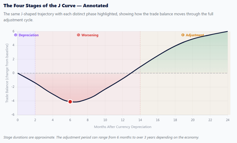
Breaking the J Curve into distinct stages makes it easier to apply to real policy situations. Each stage has a different feel — from the alarming dip to the rewarding recovery.
1. Currency Depreciation
The exchange rate falls — through market forces or deliberate policy. Trade balance unchanged at this moment.
2. Immediate Worsening
Import costs spike. Export volumes haven’t risen yet. The deficit expands — the psychologically hardest phase for policymakers.
3. Adjustment & Stabilization
Contracts expire. Businesses adapt. Foreign demand for exports slowly builds. Domestic import substitution begins.
4. Recovery & Improvement
Export volumes surge. Import volumes fall. The trade balance improves — often surpassing the pre-depreciation level.
Figure 2 · Stage Breakdown
Stages at a Glance: Comparison Table
The table below captures how eight key economic variables shift across the three broad periods of the J Curve cycle — before, during, and after the adjustment.
| Factor | Before Depreciation | During Adjustment | After Adjustment |
|---|---|---|---|
| Exchange Rate | Stable / stronger | Weakening | Stabilized at lower level |
| Import Prices | Normal | Rising sharply | Elevated but stable |
| Export Prices (foreign buyers) | Normal | Falling | Competitively low |
| Import Volume | Normal | Unchanged (contracts) | Declining |
| Export Volume | Normal | Marginally rising | Increasing significantly |
| Trade Balance | Baseline | Worsening (deficit grows) | Improving (deficit shrinks) |
| Consumer Behavior | Existing habits | Gradually shifting | Adapted to new prices |
| Business Response | Status quo | Renegotiating contracts | Realigned supply chains |
Real-World Examples of the J Curve
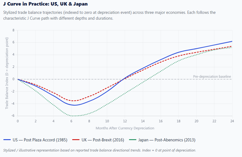
United States — The Plaza Accord (1985)
One of the most studied J Curve examples in history occurred after the Plaza Accord of September 1985, when the G5 nations agreed to deliberately weaken the US dollar. The dollar fell sharply against the Japanese yen and German mark. Yet the US trade deficit continued to widen for roughly two years before finally beginning to shrink in 1987. This delay matched the J Curve pattern almost precisely and validated the theory for a generation of economists.
United Kingdom — Post-Brexit Pound Depreciation (2016)
Following the Brexit referendum in June 2016, the British pound fell approximately 15–20% against major currencies. In the months immediately after, the UK’s trade deficit in goods actually widened, as import bills rose faster than export gains materialized. The adjustment period extended well into 2017 and beyond — a textbook J Curve playing out in real time.
Japan — Yen Depreciation Under Abenomics (2013)
When Japan embarked on aggressive monetary easing under Prime Minister Shinzo Abe in 2012–2013, the yen depreciated substantially. Initially, Japan’s trade balance deteriorated sharply — partly because Japan is heavily dependent on imported energy, which became far more expensive. The J Curve effect was more pronounced and prolonged than typical, underscoring that the theory’s timeline varies significantly across economies.
Figure 3 · Historical Comparison
Advantages and Limitations of the J Curve Theory
Advantages
- Explains real-world patterns — It accurately describes why trade deficits often worsen after a depreciation before improving.
- Guides policy expectations — It helps policymakers and investors interpret short-term data without panicking or reversing course prematurely.
- Internationally applicable — The J Curve framework has been observed in economies from the US and UK to developing nations.
- Integrates multiple economic forces — It brings together exchange rate theory, price elasticity, contract theory, and consumer behavior in one framework.
Limitations
- Timing is unpredictable — The J Curve does not specify exactly how long the initial deterioration will last. It can range from months to several years.
- Doesn’t account for structural issues — If an economy has deep structural trade problems, depreciation alone may not deliver the expected improvement.
- Energy-dependent economies face distortions — Countries reliant on imported energy (like Japan) may see the J Curve play out very differently.
- Assumes demand elasticity — The theory depends on the Marshall-Lerner condition holding, which isn’t guaranteed in all sectors.
- Global context matters — If trading partners also depreciate their currencies simultaneously, the competitive advantage may be neutralized.
J Curve vs. Other Economic Theories
The J Curve doesn’t exist in isolation. It connects to and sometimes complements several other economic frameworks.
J Curve vs. Purchasing Power Parity (PPP)
PPP suggests exchange rates eventually adjust so that identical goods cost the same across countries. The J Curve is more concerned with the transition period — the path, not the destination. They are complementary rather than contradictory.
J Curve vs. Marshall-Lerner Condition
The Marshall-Lerner condition is the mathematical foundation that determines whether a depreciation will ultimately improve the trade balance. The J Curve describes how it gets there — and the temporary detour through deterioration that occurs first.
J Curve in Private Equity
Outside macroeconomics, “J Curve” also describes how private equity funds show negative returns in early years (as fees and capital calls accumulate) before delivering strong positive returns later. The shape is identical; the underlying mechanics are entirely different.
J Curve vs. Keynesian Multiplier
Keynesian theory focuses on how government spending stimulates aggregate demand. The J Curve focuses specifically on trade responses to exchange rate movements. Both involve delays between policy action and economic outcome, but they operate through entirely different channels.
Frequently Asked Questions
Q1: What is the J Curve in simple terms? The J Curve describes the short-term worsening followed by long-term improvement in a country’s trade balance after its currency depreciates. The name comes from the shape the trade balance traces when plotted on a graph — first dipping, then rising.
Q2: How long does the J Curve effect last? The duration varies by country and circumstance, but most economists observe the initial deterioration lasting anywhere from six months to two years. The full improvement may take two to four years to materialize completely.
Q3: Does the J Curve always happen after currency depreciation? Not always. The J Curve effect is most pronounced when the Marshall-Lerner condition holds — that is, when export and import demand are sufficiently elastic. In economies with low price elasticity (such as those heavily dependent on essential imports), the curve may be shallower or take longer.
Q4: What is the difference between currency depreciation and devaluation? Depreciation refers to a market-driven decline in a currency’s value. Devaluation is a deliberate government or central bank decision to lower the official exchange rate. Both can trigger J Curve effects, but devaluation is a policy choice typically made to boost export competitiveness.
Q5: Has the United States experienced the J Curve? Yes. The most cited US example is the period following the 1985 Plaza Accord. Despite a significant dollar depreciation, the US trade deficit continued to widen into 1987 before beginning to narrow — a near-perfect real-world demonstration of the J Curve.
Q6: Is the J Curve relevant for investors? Absolutely. Investors in currency markets, multinational equities, and bonds need to understand that exchange rate movements don’t produce immediate trade effects. The J Curve explains why a depreciating currency doesn’t automatically mean improving fundamentals in the short term — and why patience is often required.
Q7: Can government policy shorten the J Curve adjustment period? To some degree. Policies that support export industries, encourage domestic production, or accelerate contract renegotiation can help compress the timeline. However, the fundamental delay caused by price-volume adjustment dynamics cannot be eliminated entirely.
Conclusion
The J Curve is one of economics’ most intuitive yet counterintuitive concepts. It tells us something important about how the real world works: change takes time, and the short-term effects of a policy action can look very different from the long-term outcomes.
For students, the J Curve is a compelling lesson in why economic models must account for lags and behavioral adjustment. For investors, it’s a reminder that deteriorating trade data after a depreciation isn’t necessarily a sign that things are getting worse — it may simply be the bottom of the curve. For policymakers, it’s both a warning and a roadmap: hold course through the dip, because the recovery is built into the pattern.
Whether you’re analyzing the US dollar, watching the British pound, or studying Japan’s monetary experiments, the J Curve framework provides a powerful lens for understanding how currency depreciation, exchange rates, and the balance of trade interact across time. Master this concept, and you’ll read trade data — and economic headlines — with far sharper eyes.