Isoquant Curve Analysis of Production in Economics

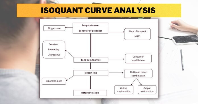
In this article, we will discuss the Isoquant curve analysis. After reading this article you will learn about:

• What is an Isoquant curve?
• What is the marginal rate of technical substitution?
• Properties of the isoquant
• Ridge line
• Consumer equilibrium under isoquant framework
• Expansion path

Let’s see.

What is an Isoquant curve?

The isoquant curve is the main tool to explain the behavior of producers. It shows the different combinations of inputs with which gives different levels of output. By using an ”isoquant approach” we can analyze the behavior of the producers in the long-run production. In this analysis, we assume that

• Producers are rational
• Level of output remains constant
• Inputs are divisible and can substitute for each other

The isoquant curve can present as an algebraic equation or as a schedule or as a graph.

In a two dimensional plane that shows two inputs, say L and K, we can mark various input combinations, which gives a different level of output.

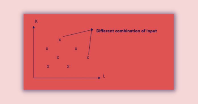
Among these various input combinations, we can identify some particular combinations which yield the same level of output. The set of these points of inputs generates the isoquant curve graphically as shown in Figure 1.

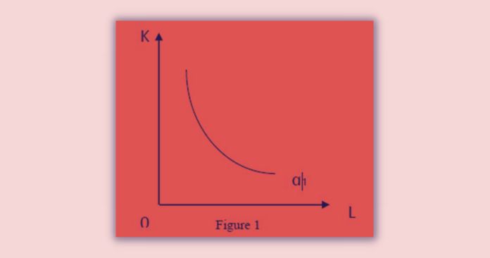
Thus, Isoquant curve can define as the locus of all possible combinations of inputs that yield a specific level of output.

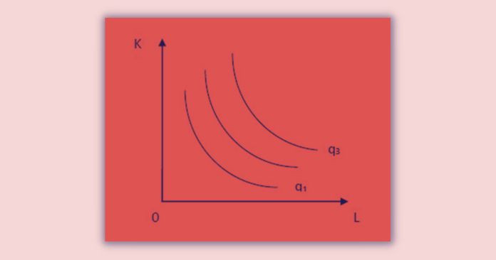
The map which includes a set of isoquant curves is called ‘isoquant map.’ In such a map, isoquants further away from the original show a higher level of output.

Isoquant Curve Analysis: What is the slope of an Isoquant?

The slope of an isoquant measures MRTS_L,K. The slope of any point of a particular isoquant is equal to the slope of the tangent drawn to that point.

What is Marginal Rate of Technical Substitution (MRTS)

MRTS is the ratio between the quantities of one input that a producer can be given up for other input in order to maintain output at the same level.

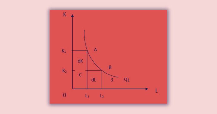
Assume that producer is at point A on the isoquant curve, which produces q₁ units by using the L₁K₁ input combination. Suppose that producer moves along the isoquant from A to B. The input combination now has changed to L₂K₂. But the output level remains the same as q₁.

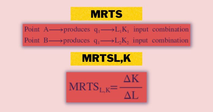
MRTS_L,K is defined as the number of units of input K that gives up in exchange for an extra unit of L. So that the producer maintains the same level of output.

Isoquant Curve Analysis: What are the Properties of the isoquant

1. Isoquant curves are downward sloping. (negative slope)

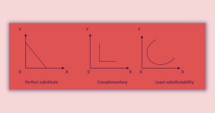
2. Isoquant of a rational producer is convex towards the origin. Also, it shows decreasing MRTS as one factor is substituted for the other.

In principle, there may be different shapes of Isoquant curves depending on the substitutability among factors. Few of such alternative shapes are given below:

3. Two isoquant cannot intersect each other.

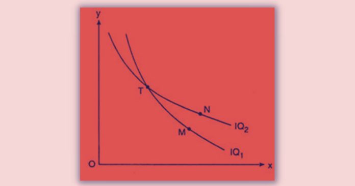
T=M (Q₁) T=N (Q₂)

According to this M must be equal to N. But (Q₁)< (Q₂)

So N>M

Ridge Lines produce in Isoquant Curve Analysis

In principle, the marginal product of factor inputs assume any value positive, negative or zero. But, the rational producer does not employ an input when its marginal product is negative.

For the production function q = f(L, K)

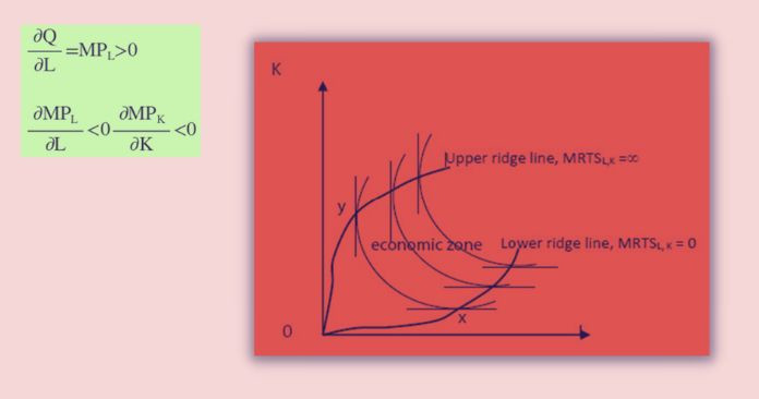
The positive range of the isoquant in the right-hand in which MP_L is negative. The left-hand side suggests that the MP_K is negative.

Ridgelines can define as the locus of points of isoquants where the marginal products of the factors are zero. Production techniques are efficient only within the ridge lines. It is called the ‘economic zone of production.’ The rational producer takes his production decisions only within this range.

This segment is identical to the second stage of short-run production.

What is Consumer equilibrium under the isoquant framework

In the analysis of the equilibrium of a rational producer under the isoquant framework,

1. we assume that the map of isoquant which ranked the desirability of production is given.
2. The outlay has been given.
3. Factor prices are determined by the factor market.
4. The goal of the producer is profit maximization.

Although the producer is willing to attain the highest level of output represent by the highest isoquant in the isoquant map, he cannot do so because his outlay is insufficient. This means that his attempt of maximizing profit is constrained by the cost of production determined by the outlay and factor prices. Thus, producer equilibrium can be considered as a constrained profit maximization problem.

Isoquant Curve Analysis: Isocost line

Suppose that the cost constraint is C₀ = wL + rK. If the quantity of L is zero, the producer could buy C₀/K quantity of K. If K is zero, he can buy C₀/L quantity of L. By including these values in a two-dimensional plane, we could form the cost constraint graphically. It is called the ‘isocost line.’

Although factor combinations along the iso-cost line are different, the cost for all combinations are the same.

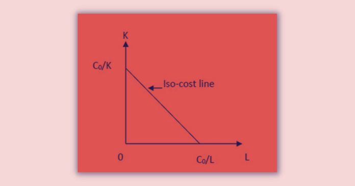
The iso-cost line is the locus of all combinations of factors the producer can purchase with a given outlay.

The slope of the iso-cost line is equal to the ratio of factor prices. (w/r)

The producer would be able to determine the optimum input combination under two approaches.

1. Constrained output maximization

The producer’s aim is to decide the optimum factor combination. So that maximize the output for the given cost constraint. In this case, assume that outlay and factor prices are given.

Max –  Q = f(L, K)

Subject to – C₀ = wL + rK

2. Constrained cost minimization

The producer’s aim is to decide the optimum factor combination. So that minimizes the cost of production for the given level of output. In this case, assume that the level of output and factor prices are given.

Min – C = wL + rK

Subject to – Q₀ = f(L, K)

Isoquant curve: Constrained output maximization

In this we assume that the isoquant map and the cost constraint are given. And also the producer knows the cost of production but not precisely the output level.

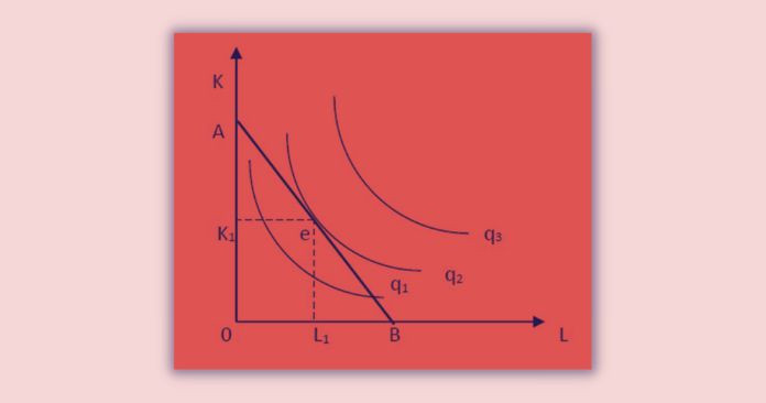
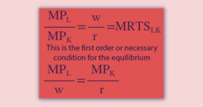
At point e,

Slope of Isoquant = Slope of Isocost

The second or sufficient condition for the equilibrium is that the isoquant must be convex to the origin at the equilibrium. If the isoquant concave at the point of tangency, it does not define as an equilibrium position.

Isoquant Curve Analysis: Constrained cost minimization

In this case, producers attempt to minimize the cost of production for the given level of output. In other words for the known quantity of output producer must determine the possible lowest cost factor combination.

The equilibrium point is the point that an iso-cost line tangent to the iso-quant which represents the given level of output.

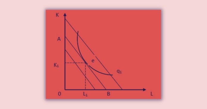
The producer is in equilibrium at point e that isocost line A-B tangent to the isoquant which gives q₁ output level.

Isoquant Curve Analysis: What is Expansion path

The equilibrium can change when factor prices or money outlay change. These changes affect the cost constraint. Assume that total outlay available increases keeping factor prices constant. In such a situation isocost line shifts upward parallelly and the equilibrium is determined at the points where it touches a higher isoquant.

The shift of the isocost line continues further with increases in money outlay. Thus producer’s equilibrium will be higher on higher isoquants. The line or curve we get by joining these equilibrium points passing through the origin called ‘expansion path’.

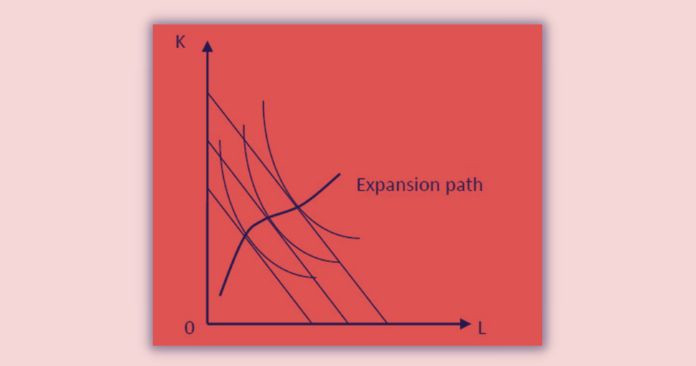
Expansion path can interpret as ‘the locus of all equilibrium points when expenditure on inputs increases keeping input prices constant.’

• The expansion path for a homogeneous PF will be a straight line.
• The expansion path for a non-homogeneous PF will be a curve.

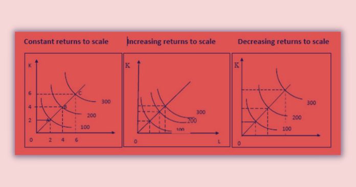
Returns to Scale in Isoquant Framework

There are three types of returns to scale in the long-run production. Returns to scale can be illustrated clearly with the use of the isoquant map. This can be done in two ways:

1. The behavior of the output level when both inputs are increased by the same proportion.

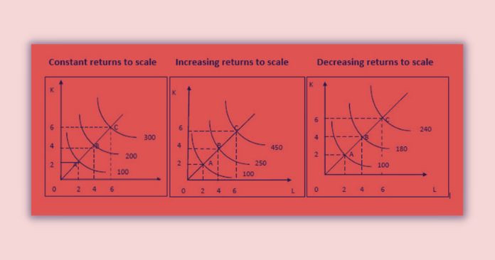
2. Considering the input required to increase the output by the same proportion.

Conclusion All right then. In this article, we discussed Isoquant curve analysis. Behavior of the producer in long-run production can analyze by using the isoquant approach. To further understand this topic follow the below topics.

Types of Isoquants in Production

Theory of Production: short-run, Long-run

Production Function: 3 Types of Production Function